XAI for Sea Ice Classification of Waveform Characteristics#
This notebook demonstrates techniques for classifying sea ice and leads from waveform data using both deep learning and tree-based methods and the ways to show which waveform characteristics contributes the most to the classification.
Models Implemented#
CNN: Captures patterns directly from raw waveforms
Random Forest: Robust ensemble approach with inherent feature importance
Gradient Boosting: Sequential learning focused on misclassification correction
XGBoost: Optimised gradient boosting with regularisation
Key Analysis Techniques#
Preprocessing of waveform characteristics
SHAP values for CNN interpretability
Model comparison with confusion matrices
Identification of consensus important regions across models
The notebook identifies which waveform characteristics are most discriminative for sea ice classification, offering insights that may improve for waveform classification.
1. Data Preprocessing#
Reads waveform data from a CSV file and processes it into structured arrays.
Handles missing values and class label inconsistencies.
Splits data into training and test sets while scaling features for consistency.
2. CNN Model for Waveform Classification#
Implements a Convolutional Neural Network (CNN) to classify sea ice and leads from radar waveform characteristics.
Uses multiple convolutional layers with batch normalisation, max pooling, dropout, and dense layers.
Compiles with the Adam optimizer and binary cross-entropy loss, monitoring performance with accuracy and AUC metrics.
Trains with early stopping and learning rate reduction strategies to prevent overfitting.
Plots training history to assess model performance over epochs.
3. Model Evaluation & Explainability (SHAP & Gradients)#
Evaluates the trained CNN model on the test set, reporting accuracy, confusion matrix, and classification metrics.
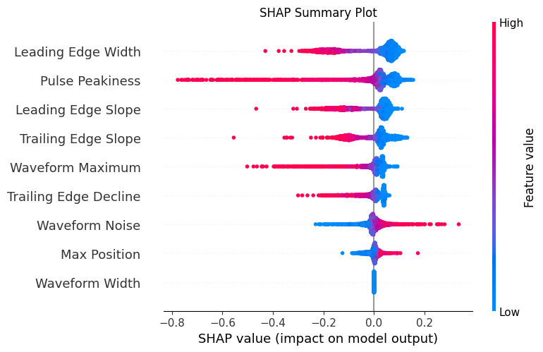
Uses SHAP (SHapley Additive Explanations) values to interpret feature importance, identifying key waveform regions influencing classification.
Helps in understanding which waveform characteristics contribute most to sea ice classification decisions.
We need to install GPY and restart session as we did in our last notebook.
!pip install Gpy
import numpy as np
import pandas as pd
import matplotlib.pyplot as plt
from sklearn.model_selection import train_test_split
from sklearn.preprocessing import StandardScaler
from sklearn.metrics import classification_report, confusion_matrix, accuracy_score, roc_curve, auc
import tensorflow as tf
from tensorflow.keras.models import Sequential
from tensorflow.keras.layers import Dense, Dropout, BatchNormalization
from tensorflow.keras.callbacks import EarlyStopping, ReduceLROnPlateau
import seaborn as sns
import ast
from scipy.optimize import curve_fit
from scipy.stats import median_abs_deviation
import shap

# Function to parse string representation of waveform array into numeric values
def parse_waveform(waveform_str):
    """Parse the string representation of waveform array into numeric values"""
    cleaned_str = waveform_str.replace('e+', 'e').replace(' ', '')

    try:
        # Use ast.literal_eval for safe evaluation of the string as a list
        waveform_list = ast.literal_eval(cleaned_str)
        return np.array(waveform_list)
    except (SyntaxError, ValueError) as e:
        try:
            # Manual parsing fallback
            values_str = waveform_str.strip('[]').split(',')
            values = []
            for val in values_str:
                val = val.strip()
                if val:  # Skip empty strings
                    values.append(float(val))
            return np.array(values)
        except Exception as e2:
            print(f"Error parsing waveform: {e2}")
            return np.array([])

# ----- Waveform Feature Extraction Functions -----

def extract_waveform_features(waveform):
    """Extract features from a radar waveform as described in the literature"""
    features = {}

    # Normalize waveform for relative measurements
    if np.max(waveform) > 0:
        norm_waveform = waveform / np.max(waveform)
    else:
        norm_waveform = waveform.copy()

    # 1. Leading Edge Width (LEW)
    # Find the positions where the waveform crosses 30% and 70% thresholds on rising edge
    try:
        # Find the maximum position
        max_idx = np.argmax(norm_waveform)

        # Find indexes before the peak where waveform crosses 30% and 70% thresholds
        thresh_30_idx = None
        thresh_70_idx = None

        for i in range(max_idx):
            if norm_waveform[i] <= 0.3 and norm_waveform[i+1] > 0.3:
                # Interpolate to find more precise bin position
                frac = (0.3 - norm_waveform[i]) / (norm_waveform[i+1] - norm_waveform[i])
                thresh_30_idx = i + frac
            if norm_waveform[i] <= 0.7 and norm_waveform[i+1] > 0.7:
                # Interpolate to find more precise bin position
                frac = (0.7 - norm_waveform[i]) / (norm_waveform[i+1] - norm_waveform[i])
                thresh_70_idx = i + frac

        # If thresholds weren't found before peak, use default values
        if thresh_30_idx is None or thresh_70_idx is None:
            features['lew'] = np.nan
        else:
            features['lew'] = thresh_70_idx - thresh_30_idx
    except:
        features['lew'] = np.nan

    # 2. Waveform Maximum (Wm)
    features['wm'] = np.max(waveform)

    # 3. Trailing Edge Decline (Ted)
    try:
        # Exponential decay function for fitting
        def exp_decay(x, a, b):
            return a * np.exp(-b * x)

        max_idx = np.argmax(waveform)
        trailing_edge = waveform[max_idx:]

        if len(trailing_edge) > 3:  # Need at least a few points for fitting
            x_data = np.arange(len(trailing_edge))

            # Avoid curve_fit errors by ensuring positive values
            trailing_edge_pos = np.maximum(trailing_edge, 1e-10)

            # Initial guess for parameters
            p0 = [trailing_edge_pos[0], 0.1]

            try:
                # Fit exponential decay to trailing edge
                popt, _ = curve_fit(exp_decay, x_data, trailing_edge_pos, p0=p0, maxfev=1000)
                features['ted'] = popt[1]  # Decay rate parameter
            except:
                features['ted'] = np.nan
        else:
            features['ted'] = np.nan
    except:
        features['ted'] = np.nan

    # 4. Waveform Noise (Wn) - MAD of trailing edge residuals
    try:
        max_idx = np.argmax(waveform)
        trailing_edge = waveform[max_idx:]

        if len(trailing_edge) > 3 and 'ted' in features and not np.isnan(features['ted']):
            # Using the fitted parameters from Ted
            x_data = np.arange(len(trailing_edge))
            fitted_values = features['wm'] * np.exp(-features['ted'] * x_data)

            # Calculate residuals
            residuals = trailing_edge - fitted_values

            # MAD of residuals
            features['wn'] = median_abs_deviation(residuals, scale=1.0)
        else:
            features['wn'] = np.nan
    except:
        features['wn'] = np.nan

    # 5. Waveform Width (Ww)
    # Count bins with power > 0
    features['ww'] = np.sum(waveform > 0)

    # 6. Leading Edge Slope (Les)
    try:
        max_idx = np.argmax(norm_waveform)

        # Find bins where waveform exceeds 30% of max
        thresh_30_idx = None
        for i in range(max_idx):
            if norm_waveform[i] <= 0.3 and norm_waveform[i+1] > 0.3:
                thresh_30_idx = i
                break

        if thresh_30_idx is not None:
            # Calculate difference between max bin and first 30% threshold bin
            features['les'] = max_idx - thresh_30_idx
        else:
            features['les'] = np.nan
    except:
        features['les'] = np.nan

    # 7. Trailing Edge Slope (Tes)
    try:
        max_idx = np.argmax(norm_waveform)

        # Find last bin where waveform exceeds 30% of max
        thresh_30_idx = None
        for i in range(len(norm_waveform)-1, max_idx, -1):
            if norm_waveform[i] <= 0.3 and norm_waveform[i-1] > 0.3:
                thresh_30_idx = i
                break

        if thresh_30_idx is not None:
            # Calculate difference between last 30% threshold bin and max bin
            features['tes'] = thresh_30_idx - max_idx
        else:
            features['tes'] = np.nan
    except:
        features['tes'] = np.nan

    # 8. Pulse Peakiness (PP) - common waveform feature in literature
    try:
        features['pp'] = features['wm'] / np.mean(waveform)
    except:
        features['pp'] = np.nan

    # 9. Max position (relative bin where the maximum occurs)
    try:
        features['max_pos'] = np.argmax(waveform) / len(waveform)
    except:
        features['max_pos'] = np.nan

    return features

def extract_waveforms_and_features(roughness, target_column):
    """Process all waveforms and extract features"""
    # Lists to store data
    feature_list = []
    target_list = []
    valid_indices = []
    raw_waveforms = []

    print("Extracting features from waveforms...")

    # Process each row
    for idx, row in roughness.iterrows():
        if idx % 500 == 0:
            print(f"Processing row {idx}/{len(roughness)}...")

        try:
            # Get the waveform and class
            waveform_str = str(row['Matched_Waveform_20_Ku'])
            waveform_array = parse_waveform(waveform_str)

            # Get class label
            class_label = int(row[target_column])

            # Extract features if valid waveform
            if len(waveform_array) > 0:
                # Extract features
                features = extract_waveform_features(waveform_array)

                # Skip if any feature is NaN
                if np.any(np.isnan(list(features.values()))):
                    continue

                # Store data
                feature_list.append(list(features.values()))
                target_list.append(class_label)
                valid_indices.append(idx)
                raw_waveforms.append(waveform_array)

        except Exception as e:
            if idx < 5:  # Print first few errors
                print(f"Error processing row {idx}: {e}")
            continue

    # Convert to numpy arrays
    X_features = np.array(feature_list)
    y = np.array(target_list)
    X_raw = np.array(raw_waveforms)

    # Create feature names
    feature_names = ['Leading Edge Width', 'Waveform Maximum',
                     'Trailing Edge Decline', 'Waveform Noise',
                     'Waveform Width', 'Leading Edge Slope',
                     'Trailing Edge Slope', 'Pulse Peakiness',
                     'Max Position']

    return X_features, y, X_raw, valid_indices, feature_names
# ----- Main Processing -----
roughness = pd.read_csv('/content/drive/MyDrive/GEOL0069/2324/Week 9 2025/updated_filtered_matched_uit_sentinel3_L2_alongtrack_2023_04_official.txt')
print(roughness)
print("Starting waveform feature extraction and classification...")

# Define the target column
target_column = 'Sea_Ice_Class'
if target_column not in roughness.columns:
    print(f"Warning: {target_column} not found. Available columns: {roughness.columns}")
    print("Will use 'Lead_Class' as target instead.")
    target_column = 'Lead_Class'

# Extract features from all waveforms
X_features, y, X_raw, valid_indices, feature_names = extract_waveforms_and_features(roughness, target_column)

print(f"Extracted {len(feature_names)} features from {len(X_features)} valid waveforms")
print(f"Features: {feature_names}")
print(f"Feature data shape: {X_features.shape}")
print(f"Class distribution: {np.bincount(y)}")

# Check for NaN values
nan_mask = np.isnan(X_features).any(axis=1)
X_features_clean = X_features[~nan_mask]
y_clean = y[~nan_mask]
X_raw_clean = X_raw[~nan_mask]

print(f"Removed {np.sum(nan_mask)} samples with NaN values")
print(f"Clean feature data shape: {X_features_clean.shape}")

# Split data into training and test sets
X_train, X_test, y_train, y_test, X_raw_train, X_raw_test = train_test_split(
    X_features_clean, y_clean, X_raw_clean,
    test_size=0.2, random_state=42, stratify=y_clean
)

# Scale features
scaler = StandardScaler()
X_train_scaled = scaler.fit_transform(X_train)
X_test_scaled = scaler.transform(X_test)
       3A=0_3B=1  Orbit_#  Segment_#     Datenumber   Latitude  Longitude  \
0              0        1          1  738977.028790  74.432732 -73.103512
1              0        1          1  738977.028790  74.435182 -73.109831
2              0        1          1  738977.028791  74.437633 -73.116151
3              0        1          1  738977.028791  74.440083 -73.122474
4              0        1          1  738977.028792  74.442533 -73.128797
...          ...      ...        ...            ...        ...        ...
28720          0      843        843  739006.699439  71.763165 -74.486482
28721          0      843        843  739006.699440  71.760574 -74.491177
28722          0      843        843  739006.699440  71.757982 -74.495872
28723          0      843        843  739006.699450  71.711313 -74.580159
28724          0      843        843  739006.699451  71.708719 -74.584830

       Radar_Freeboard  Surface_Height_WGS84  Sea_Surface_Height_Interp_WGS84  \
0            -0.044136             14.319994                        14.364129
1            -0.099506             14.265998                        14.365504
2             0.029215             14.396251                        14.367035
3             0.062597             14.431502                        14.368905
4            -0.044797             14.326136                        14.370932
...                ...                   ...                              ...
28720         0.362561              0.308307                        -0.054254
28721         0.276995              0.205567                        -0.071428
28722         0.301225              0.211470                        -0.089755
28723         0.165803             -0.241391                        -0.407193
28724         0.255920             -0.165441                        -0.421361

       SSH_Uncertainty  ...  Lead_Class  Sea_Ice_Roughness  \
0             0.000254  ...           0           0.017885
1             0.000232  ...           0           0.003315
2             0.000212  ...           0           0.018211
3             0.000192  ...           0           0.051418
4             0.000173  ...           0           0.046983
...                ...  ...         ...                ...
28720         0.014538  ...           0           0.067003
28721         0.014706  ...           0           0.040842
28722         0.014876  ...           0           0.034679
28723         0.018095  ...           0           0.443806
28724         0.018284  ...           0           0.058687

       Sea_Ice_Concentration  Seconds_since_2000  Year  Month  Day  \
0                     1.0000        7.336249e+08  2023      4    1
1                     1.0000        7.336249e+08  2023      4    1
2                     1.0000        7.336249e+08  2023      4    1
3                     1.0000        7.336249e+08  2023      4    1
4                     1.0000        7.336249e+08  2023      4    1
...                      ...                 ...   ...    ...  ...
28720                 0.9083        7.361884e+08  2023      4   30
28721                 0.9083        7.361884e+08  2023      4   30
28722                 0.9083        7.361884e+08  2023      4   30
28723                 0.9083        7.361884e+08  2023      4   30
28724                 0.9083        7.361884e+08  2023      4   30

              Proj_X        Proj_Y  \
0      646585.001913  8.269660e+06
1      646373.758053  8.269917e+06
2      646162.531358  8.270174e+06
3      645951.280450  8.270431e+06
4      645740.085773  8.270688e+06
...              ...           ...
28720  622709.601630  7.969277e+06
28721  622562.605479  7.968979e+06
28722  622415.569925  7.968680e+06
28723  619768.967681  7.963311e+06
28724  619621.913813  7.963013e+06

                                  Matched_Waveform_20_Ku
0      [2.524e+00,2.780e+00,2.194e+00,2.286e+00,2.054...
1      [2.381e+00,2.182e+00,2.332e+00,2.352e+00,1.857...
2      [2.173e+00,1.961e+00,2.388e+00,2.075e+00,2.609...
3      [2.202e+00,2.223e+00,2.049e+00,2.213e+00,2.138...
4      [3.252e+00,2.874e+00,2.988e+00,2.789e+00,2.546...
...                                                  ...
28720                                                NaN
28721                                                NaN
28722                                                NaN
28723                                                NaN
28724                                                NaN

[28725 rows x 23 columns]
Starting waveform feature extraction and classification...
Extracting features from waveforms...
Processing row 0/28725...
Processing row 500/28725...
Processing row 1000/28725...
Processing row 1500/28725...
Processing row 2000/28725...
Processing row 2500/28725...
Processing row 3000/28725...
Processing row 3500/28725...
Processing row 4000/28725...
Processing row 4500/28725...
Processing row 5000/28725...
Processing row 5500/28725...
Processing row 6000/28725...
Processing row 6500/28725...
Processing row 7000/28725...
Processing row 7500/28725...
Processing row 8000/28725...
Processing row 8500/28725...
Processing row 9000/28725...
Processing row 9500/28725...
Processing row 10000/28725...
Processing row 10500/28725...
Processing row 11000/28725...
Processing row 11500/28725...
Processing row 12000/28725...
Processing row 12500/28725...
Processing row 13000/28725...
Processing row 13500/28725...
Processing row 14000/28725...
Processing row 14500/28725...
Processing row 15000/28725...
Processing row 15500/28725...
Processing row 16000/28725...
Processing row 16500/28725...
Processing row 17000/28725...
Processing row 17500/28725...
Processing row 18000/28725...
Processing row 18500/28725...
Processing row 19000/28725...
Processing row 19500/28725...
Processing row 20000/28725...
Processing row 20500/28725...
Processing row 21000/28725...
Processing row 21500/28725...
Processing row 22000/28725...
Processing row 22500/28725...
Processing row 23000/28725...
Processing row 23500/28725...
Processing row 24000/28725...
Processing row 24500/28725...
Processing row 25000/28725...
Processing row 25500/28725...
Processing row 26000/28725...
Processing row 26500/28725...
Processing row 27000/28725...
Processing row 27500/28725...
Processing row 28000/28725...
Processing row 28500/28725...
Extracted 9 features from 12765 valid waveforms
Features: ['Leading Edge Width', 'Waveform Maximum', 'Trailing Edge Decline', 'Waveform Noise', 'Waveform Width', 'Leading Edge Slope', 'Trailing Edge Slope', 'Pulse Peakiness', 'Max Position']
Feature data shape: (12765, 9)
Class distribution: [  604 12161]
Removed 0 samples with NaN values
Clean feature data shape: (12765, 9)
# ----- Neural Network Model for Feature-Based Classification -----
# Build a simple neural network model
model = Sequential([
Dense(16, activation='relu', input_shape=(X_train_scaled.shape[1],)),
BatchNormalization(),
Dropout(0.3),
Dense(8, activation='relu'),
Dropout(0.2),
Dense(1, activation='sigmoid')
])
# Compile the model
model.compile(
optimizer='adam',
loss='binary_crossentropy',
metrics=['accuracy', tf.keras.metrics.AUC()]
)
# Model summary
model.summary()
# Callbacks
callbacks = [
EarlyStopping(monitor='val_loss', patience=15, restore_best_weights=True),
ReduceLROnPlateau(monitor='val_loss', factor=0.5, patience=5, min_lr=0.0001)
]
# Apply class weights if imbalanced
class_weights = None
if len(np.unique(y_train)) > 1:
n_samples = len(y_train)
n_classes = len(np.unique(y_train))
class_counts = np.bincount(y_train)
if np.min(class_counts) / np.max(class_counts) < 0.5: # If imbalanced
print("Detected class imbalance, applying class weights")
class_weights = {i: n_samples / (n_classes * count) for i, count in enumerate(class_counts)}
# Train the model
print("\nTraining neural network model...")
history = model.fit(
X_train_scaled, y_train,
epochs=50,
batch_size=32,
validation_split=0.2,
callbacks=callbacks,
class_weight=class_weights,
verbose=1
)
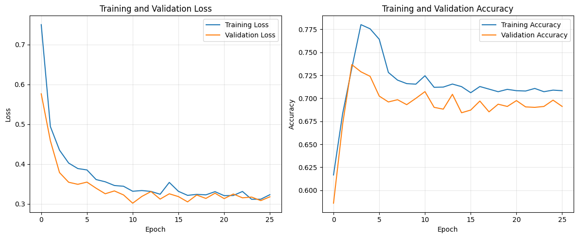
# Plot training history
plt.figure(figsize=(12, 5))
plt.subplot(1, 2, 1)
plt.plot(history.history['loss'], label='Training Loss')
plt.plot(history.history['val_loss'], label='Validation Loss')
plt.title('Training and Validation Loss')
plt.xlabel('Epoch')
plt.ylabel('Loss')
plt.legend()
plt.grid(True, alpha=0.3)
plt.subplot(1, 2, 2)
plt.plot(history.history['accuracy'], label='Training Accuracy')
plt.plot(history.history['val_accuracy'], label='Validation Accuracy')
plt.title('Training and Validation Accuracy')
plt.xlabel('Epoch')
plt.ylabel('Accuracy')
plt.legend()
plt.grid(True, alpha=0.3)
plt.tight_layout()
plt.show()
# ----- Model Evaluation -----
y_pred_prob = model.predict(X_test_scaled).flatten()
y_pred = (y_pred_prob > 0.5).astype(int)
accuracy = accuracy_score(y_test, y_pred)
print(f"\nAccuracy: {accuracy:.4f}")
print("\nClassification Report:")
print(classification_report(y_test, y_pred))
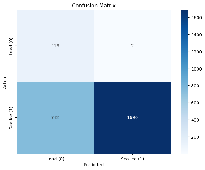
conf_matrix = confusion_matrix(y_test, y_pred)
plt.figure(figsize=(8, 6))
sns.heatmap(conf_matrix, annot=True, fmt='d', cmap='Blues',
xticklabels=['Lead (0)', 'Sea Ice (1)'],
yticklabels=['Lead (0)', 'Sea Ice (1)'])
plt.xlabel('Predicted')
plt.ylabel('Actual')
plt.title('Confusion Matrix')
plt.show()
       3A=0_3B=1  Orbit_#  Segment_#     Datenumber   Latitude  Longitude  \
0              0        1          1  738977.028790  74.432732 -73.103512
1              0        1          1  738977.028790  74.435182 -73.109831
2              0        1          1  738977.028791  74.437633 -73.116151
3              0        1          1  738977.028791  74.440083 -73.122474
4              0        1          1  738977.028792  74.442533 -73.128797
...          ...      ...        ...            ...        ...        ...
28720          0      843        843  739006.699439  71.763165 -74.486482
28721          0      843        843  739006.699440  71.760574 -74.491177
28722          0      843        843  739006.699440  71.757982 -74.495872
28723          0      843        843  739006.699450  71.711313 -74.580159
28724          0      843        843  739006.699451  71.708719 -74.584830

       Radar_Freeboard  Surface_Height_WGS84  Sea_Surface_Height_Interp_WGS84  \
0            -0.044136             14.319994                        14.364129
1            -0.099506             14.265998                        14.365504
2             0.029215             14.396251                        14.367035
3             0.062597             14.431502                        14.368905
4            -0.044797             14.326136                        14.370932
...                ...                   ...                              ...
28720         0.362561              0.308307                        -0.054254
28721         0.276995              0.205567                        -0.071428
28722         0.301225              0.211470                        -0.089755
28723         0.165803             -0.241391                        -0.407193
28724         0.255920             -0.165441                        -0.421361

       SSH_Uncertainty  ...  Lead_Class  Sea_Ice_Roughness  \
0             0.000254  ...           0           0.017885
1             0.000232  ...           0           0.003315
2             0.000212  ...           0           0.018211
3             0.000192  ...           0           0.051418
4             0.000173  ...           0           0.046983
...                ...  ...         ...                ...
28720         0.014538  ...           0           0.067003
28721         0.014706  ...           0           0.040842
28722         0.014876  ...           0           0.034679
28723         0.018095  ...           0           0.443806
28724         0.018284  ...           0           0.058687

       Sea_Ice_Concentration  Seconds_since_2000  Year  Month  Day  \
0                     1.0000        7.336249e+08  2023      4    1
1                     1.0000        7.336249e+08  2023      4    1
2                     1.0000        7.336249e+08  2023      4    1
3                     1.0000        7.336249e+08  2023      4    1
4                     1.0000        7.336249e+08  2023      4    1
...                      ...                 ...   ...    ...  ...
28720                 0.9083        7.361884e+08  2023      4   30
28721                 0.9083        7.361884e+08  2023      4   30
28722                 0.9083        7.361884e+08  2023      4   30
28723                 0.9083        7.361884e+08  2023      4   30
28724                 0.9083        7.361884e+08  2023      4   30

              Proj_X        Proj_Y  \
0      646585.001913  8.269660e+06
1      646373.758053  8.269917e+06
2      646162.531358  8.270174e+06
3      645951.280450  8.270431e+06
4      645740.085773  8.270688e+06
...              ...           ...
28720  622709.601630  7.969277e+06
28721  622562.605479  7.968979e+06
28722  622415.569925  7.968680e+06
28723  619768.967681  7.963311e+06
28724  619621.913813  7.963013e+06

                                  Matched_Waveform_20_Ku
0      [2.524e+00,2.780e+00,2.194e+00,2.286e+00,2.054...
1      [2.381e+00,2.182e+00,2.332e+00,2.352e+00,1.857...
2      [2.173e+00,1.961e+00,2.388e+00,2.075e+00,2.609...
3      [2.202e+00,2.223e+00,2.049e+00,2.213e+00,2.138...
4      [3.252e+00,2.874e+00,2.988e+00,2.789e+00,2.546...
...                                                  ...
28720                                                NaN
28721                                                NaN
28722                                                NaN
28723                                                NaN
28724                                                NaN

[28725 rows x 23 columns]
Starting waveform feature extraction and classification...
Extracting features from waveforms...
Processing row 0/28725...
Processing row 500/28725...
Processing row 1000/28725...
Processing row 1500/28725...
Processing row 2000/28725...
Processing row 2500/28725...
Processing row 3000/28725...
Processing row 3500/28725...
Processing row 4000/28725...
Processing row 4500/28725...
Processing row 5000/28725...
Processing row 5500/28725...
Processing row 6000/28725...
Processing row 6500/28725...
Processing row 7000/28725...
Processing row 7500/28725...
Processing row 8000/28725...
Processing row 8500/28725...
Processing row 9000/28725...
Processing row 9500/28725...
Processing row 10000/28725...
Processing row 10500/28725...
Processing row 11000/28725...
Processing row 11500/28725...
Processing row 12000/28725...
Processing row 12500/28725...
Processing row 13000/28725...
Processing row 13500/28725...
Processing row 14000/28725...
Processing row 14500/28725...
Processing row 15000/28725...
Processing row 15500/28725...
Processing row 16000/28725...
Processing row 16500/28725...
Processing row 17000/28725...
Processing row 17500/28725...
Processing row 18000/28725...
Processing row 18500/28725...
Processing row 19000/28725...
Processing row 19500/28725...
Processing row 20000/28725...
Processing row 20500/28725...
Processing row 21000/28725...
Processing row 21500/28725...
Processing row 22000/28725...
Processing row 22500/28725...
Processing row 23000/28725...
Processing row 23500/28725...
Processing row 24000/28725...
Processing row 24500/28725...
Processing row 25000/28725...
Processing row 25500/28725...
Processing row 26000/28725...
Processing row 26500/28725...
Processing row 27000/28725...
Processing row 27500/28725...
Processing row 28000/28725...
Processing row 28500/28725...
Extracted 9 features from 12765 valid waveforms
Features: ['Leading Edge Width', 'Waveform Maximum', 'Trailing Edge Decline', 'Waveform Noise', 'Waveform Width', 'Leading Edge Slope', 'Trailing Edge Slope', 'Pulse Peakiness', 'Max Position']
Feature data shape: (12765, 9)
Class distribution: [  604 12161]
Removed 0 samples with NaN values
Clean feature data shape: (12765, 9)
/usr/local/lib/python3.11/dist-packages/keras/src/layers/core/dense.py:87: UserWarning: Do not pass an `input_shape`/`input_dim` argument to a layer. When using Sequential models, prefer using an `Input(shape)` object as the first layer in the model instead.
  super().__init__(activity_regularizer=activity_regularizer, **kwargs)
Model: "sequential_1"
┏━━━━━━━━━━━━━━━━━━━━━━━━━━━━━━━━━━━━━━┳━━━━━━━━━━━━━━━━━━━━━━━━━━━━━┳━━━━━━━━━━━━━━━━━┓
┃ Layer (type)                         ┃ Output Shape                ┃         Param # ┃
┡━━━━━━━━━━━━━━━━━━━━━━━━━━━━━━━━━━━━━━╇━━━━━━━━━━━━━━━━━━━━━━━━━━━━━╇━━━━━━━━━━━━━━━━━┩
│ dense_4 (Dense)                      │ (None, 16)                  │             160 │
├──────────────────────────────────────┼─────────────────────────────┼─────────────────┤
│ batch_normalization_1                │ (None, 16)                  │              64 │
│ (BatchNormalization)                 │                             │                 │
├──────────────────────────────────────┼─────────────────────────────┼─────────────────┤
│ dropout_2 (Dropout)                  │ (None, 16)                  │               0 │
├──────────────────────────────────────┼─────────────────────────────┼─────────────────┤
│ dense_5 (Dense)                      │ (None, 8)                   │             136 │
├──────────────────────────────────────┼─────────────────────────────┼─────────────────┤
│ dropout_3 (Dropout)                  │ (None, 8)                   │               0 │
├──────────────────────────────────────┼─────────────────────────────┼─────────────────┤
│ dense_6 (Dense)                      │ (None, 1)                   │               9 │
└──────────────────────────────────────┴─────────────────────────────┴─────────────────┘
Total params: 369 (1.44 KB)
Trainable params: 337 (1.32 KB)
Non-trainable params: 32 (128.00 B)
Detected class imbalance, applying class weights

Training neural network model...
Epoch 1/50
256/256 ━━━━━━━━━━━━━━━━━━━━ 7s 14ms/step - accuracy: 0.5987 - auc_1: 0.5160 - loss: 1.0171 - val_accuracy: 0.5859 - val_auc_1: 0.9090 - val_loss: 0.5763 - learning_rate: 0.0010
Epoch 2/50
256/256 ━━━━━━━━━━━━━━━━━━━━ 1s 3ms/step - accuracy: 0.6790 - auc_1: 0.8197 - loss: 0.5255 - val_accuracy: 0.6721 - val_auc_1: 0.9266 - val_loss: 0.4585 - learning_rate: 0.0010
Epoch 3/50
256/256 ━━━━━━━━━━━━━━━━━━━━ 1s 4ms/step - accuracy: 0.7154 - auc_1: 0.8620 - loss: 0.4470 - val_accuracy: 0.7367 - val_auc_1: 0.9282 - val_loss: 0.3785 - learning_rate: 0.0010
Epoch 4/50
256/256 ━━━━━━━━━━━━━━━━━━━━ 1s 3ms/step - accuracy: 0.7772 - auc_1: 0.8951 - loss: 0.4121 - val_accuracy: 0.7288 - val_auc_1: 0.9296 - val_loss: 0.3542 - learning_rate: 0.0010
Epoch 5/50
256/256 ━━━━━━━━━━━━━━━━━━━━ 1s 4ms/step - accuracy: 0.7839 - auc_1: 0.9084 - loss: 0.3748 - val_accuracy: 0.7239 - val_auc_1: 0.9302 - val_loss: 0.3491 - learning_rate: 0.0010
Epoch 6/50
256/256 ━━━━━━━━━━━━━━━━━━━━ 1s 3ms/step - accuracy: 0.7602 - auc_1: 0.9008 - loss: 0.3841 - val_accuracy: 0.7024 - val_auc_1: 0.9261 - val_loss: 0.3546 - learning_rate: 0.0010
Epoch 7/50
256/256 ━━━━━━━━━━━━━━━━━━━━ 1s 5ms/step - accuracy: 0.7219 - auc_1: 0.9073 - loss: 0.3571 - val_accuracy: 0.6960 - val_auc_1: 0.9287 - val_loss: 0.3392 - learning_rate: 0.0010
Epoch 8/50
256/256 ━━━━━━━━━━━━━━━━━━━━ 1s 5ms/step - accuracy: 0.7216 - auc_1: 0.9023 - loss: 0.3778 - val_accuracy: 0.6985 - val_auc_1: 0.9304 - val_loss: 0.3253 - learning_rate: 0.0010
Epoch 9/50
256/256 ━━━━━━━━━━━━━━━━━━━━ 1s 4ms/step - accuracy: 0.7148 - auc_1: 0.9115 - loss: 0.3437 - val_accuracy: 0.6931 - val_auc_1: 0.9301 - val_loss: 0.3325 - learning_rate: 0.0010
Epoch 10/50
256/256 ━━━━━━━━━━━━━━━━━━━━ 1s 3ms/step - accuracy: 0.7191 - auc_1: 0.9179 - loss: 0.3579 - val_accuracy: 0.7000 - val_auc_1: 0.9325 - val_loss: 0.3224 - learning_rate: 0.0010
Epoch 11/50
256/256 ━━━━━━━━━━━━━━━━━━━━ 1s 4ms/step - accuracy: 0.7230 - auc_1: 0.9275 - loss: 0.3244 - val_accuracy: 0.7073 - val_auc_1: 0.9335 - val_loss: 0.3016 - learning_rate: 0.0010
Epoch 12/50
256/256 ━━━━━━━━━━━━━━━━━━━━ 1s 3ms/step - accuracy: 0.7053 - auc_1: 0.9204 - loss: 0.3358 - val_accuracy: 0.6902 - val_auc_1: 0.9337 - val_loss: 0.3186 - learning_rate: 0.0010
Epoch 13/50
256/256 ━━━━━━━━━━━━━━━━━━━━ 1s 4ms/step - accuracy: 0.7208 - auc_1: 0.9276 - loss: 0.3272 - val_accuracy: 0.6882 - val_auc_1: 0.9304 - val_loss: 0.3309 - learning_rate: 0.0010
Epoch 14/50
256/256 ━━━━━━━━━━━━━━━━━━━━ 1s 4ms/step - accuracy: 0.7141 - auc_1: 0.9289 - loss: 0.3243 - val_accuracy: 0.7044 - val_auc_1: 0.9376 - val_loss: 0.3119 - learning_rate: 0.0010
Epoch 15/50
256/256 ━━━━━━━━━━━━━━━━━━━━ 1s 4ms/step - accuracy: 0.7205 - auc_1: 0.9120 - loss: 0.3443 - val_accuracy: 0.6843 - val_auc_1: 0.9323 - val_loss: 0.3252 - learning_rate: 0.0010
Epoch 16/50
256/256 ━━━━━━━━━━━━━━━━━━━━ 1s 4ms/step - accuracy: 0.7030 - auc_1: 0.9160 - loss: 0.3447 - val_accuracy: 0.6872 - val_auc_1: 0.9353 - val_loss: 0.3182 - learning_rate: 0.0010
Epoch 17/50
256/256 ━━━━━━━━━━━━━━━━━━━━ 1s 4ms/step - accuracy: 0.7090 - auc_1: 0.9258 - loss: 0.3164 - val_accuracy: 0.6970 - val_auc_1: 0.9358 - val_loss: 0.3050 - learning_rate: 5.0000e-04
Epoch 18/50
256/256 ━━━━━━━━━━━━━━━━━━━━ 1s 5ms/step - accuracy: 0.7129 - auc_1: 0.9254 - loss: 0.3153 - val_accuracy: 0.6853 - val_auc_1: 0.9327 - val_loss: 0.3222 - learning_rate: 5.0000e-04
Epoch 19/50
256/256 ━━━━━━━━━━━━━━━━━━━━ 1s 5ms/step - accuracy: 0.7125 - auc_1: 0.9290 - loss: 0.3093 - val_accuracy: 0.6936 - val_auc_1: 0.9363 - val_loss: 0.3136 - learning_rate: 5.0000e-04
Epoch 20/50
256/256 ━━━━━━━━━━━━━━━━━━━━ 1s 4ms/step - accuracy: 0.7094 - auc_1: 0.9136 - loss: 0.3430 - val_accuracy: 0.6911 - val_auc_1: 0.9364 - val_loss: 0.3267 - learning_rate: 5.0000e-04
Epoch 21/50
256/256 ━━━━━━━━━━━━━━━━━━━━ 1s 3ms/step - accuracy: 0.7106 - auc_1: 0.9217 - loss: 0.3138 - val_accuracy: 0.6975 - val_auc_1: 0.9386 - val_loss: 0.3131 - learning_rate: 5.0000e-04
Epoch 22/50
256/256 ━━━━━━━━━━━━━━━━━━━━ 1s 3ms/step - accuracy: 0.7096 - auc_1: 0.9174 - loss: 0.3282 - val_accuracy: 0.6907 - val_auc_1: 0.9359 - val_loss: 0.3247 - learning_rate: 2.5000e-04
Epoch 23/50
256/256 ━━━━━━━━━━━━━━━━━━━━ 1s 3ms/step - accuracy: 0.7119 - auc_1: 0.9241 - loss: 0.3325 - val_accuracy: 0.6902 - val_auc_1: 0.9373 - val_loss: 0.3151 - learning_rate: 2.5000e-04
Epoch 24/50
256/256 ━━━━━━━━━━━━━━━━━━━━ 1s 3ms/step - accuracy: 0.7017 - auc_1: 0.9295 - loss: 0.3036 - val_accuracy: 0.6911 - val_auc_1: 0.9370 - val_loss: 0.3170 - learning_rate: 2.5000e-04
Epoch 25/50
256/256 ━━━━━━━━━━━━━━━━━━━━ 1s 4ms/step - accuracy: 0.7080 - auc_1: 0.9372 - loss: 0.2912 - val_accuracy: 0.6980 - val_auc_1: 0.9383 - val_loss: 0.3081 - learning_rate: 2.5000e-04
Epoch 26/50
256/256 ━━━━━━━━━━━━━━━━━━━━ 1s 4ms/step - accuracy: 0.7060 - auc_1: 0.9212 - loss: 0.3306 - val_accuracy: 0.6911 - val_auc_1: 0.9385 - val_loss: 0.3177 - learning_rate: 2.5000e-04
80/80 ━━━━━━━━━━━━━━━━━━━━ 0s 3ms/step

Accuracy: 0.7086

Classification Report:
              precision    recall  f1-score   support

           0       0.14      0.98      0.24       121
           1       1.00      0.69      0.82      2432

    accuracy                           0.71      2553
   macro avg       0.57      0.84      0.53      2553
weighted avg       0.96      0.71      0.79      2553
# ----- Feature Importance Analysis -----
# Use SHAP for feature importance
print("\nCalculating feature importance using SHAP values...")
try:
# Create an explainer for the model
explainer = shap.Explainer(model, X_train_scaled)
shap_values = explainer(X_test_scaled)
# Get mean absolute SHAP values for feature importance
feature_importance = np.abs(shap_values.values).mean(0)
# Create a DataFrame for better visualization
importance_df = pd.DataFrame({
'Feature': feature_names,
'Importance': feature_importance
}).sort_values('Importance', ascending=False)
print("\nFeature Importance Ranking:")
for idx, row in importance_df.iterrows():
print(f"{row['Feature']}: {row['Importance']:.4f}")
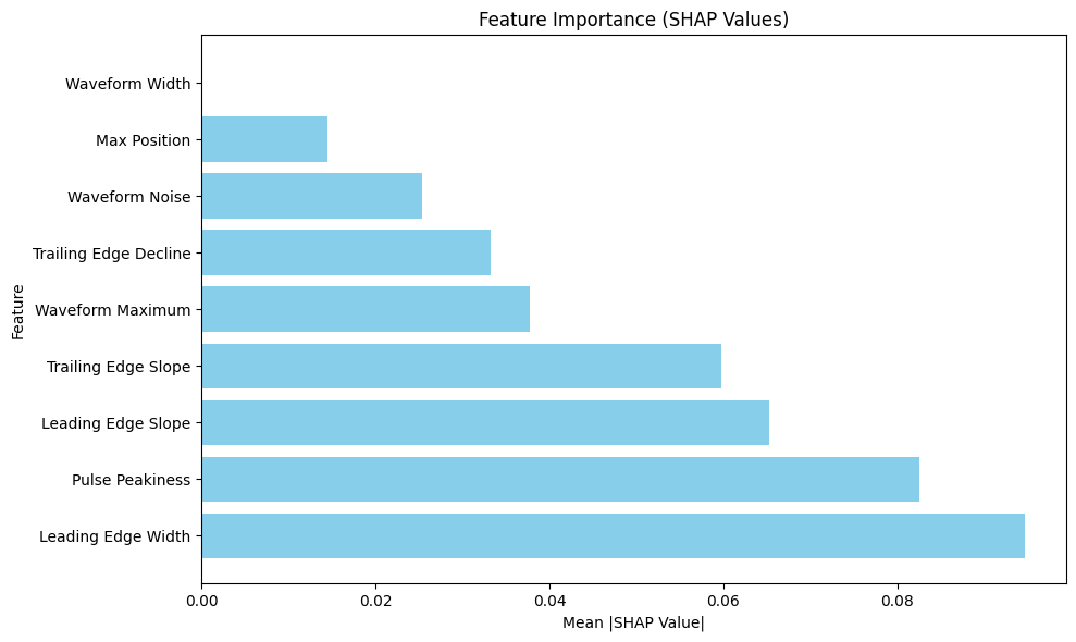
# Plot feature importance
plt.figure(figsize=(10, 6))
plt.barh(importance_df['Feature'], importance_df['Importance'], color='skyblue')
plt.xlabel('Mean |SHAP Value|')
plt.ylabel('Feature')
plt.title('Feature Importance (SHAP Values)')
plt.tight_layout()
plt.show()
# Plot SHAP summary plot (this shows direction of impact too)
plt.figure(figsize=(12, 8))
shap.summary_plot(shap_values, X_test_scaled, feature_names=feature_names, show=False)
plt.title('SHAP Summary Plot')
plt.tight_layout()
plt.show()
except Exception as e:
print(f"Error calculating SHAP values: {e}")
# Simple feature importance from model weights (for dense layers)
# This is a simpler approach that works when SHAP fails
weights = model.layers[0].get_weights()[0]
importance = np.abs(weights).mean(axis=1)
# Create a DataFrame for better visualization
importance_df = pd.DataFrame({
'Feature': feature_names,
'Importance': importance
}).sort_values('Importance', ascending=False)
print("\nFeature Importance Ranking (from model weights):")
for idx, row in importance_df.iterrows():
print(f"{row['Feature']}: {row['Importance']:.4f}")
# Plot feature importance
plt.figure(figsize=(10, 6))
plt.barh(importance_df['Feature'], importance_df['Importance'], color='skyblue')
plt.xlabel('Absolute Weight Magnitude')
plt.ylabel('Feature')
plt.title('Feature Importance (Neural Network Weights)')
plt.tight_layout()
plt.show()
print("Waveform feature-based classification complete!")
Calculating feature importance using SHAP values...
ExactExplainer explainer: 2554it [00:45, 46.92it/s]
Feature Importance Ranking:
Leading Edge Width: 0.0947
Pulse Peakiness: 0.0826
Leading Edge Slope: 0.0653
Trailing Edge Slope: 0.0598
Waveform Maximum: 0.0378
Trailing Edge Decline: 0.0332
Waveform Noise: 0.0253
Max Position: 0.0145
Waveform Width: 0.0000
Waveform feature-based classification complete!
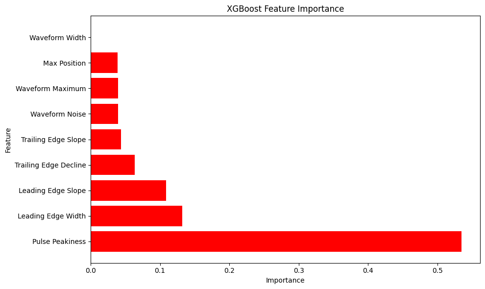
4. Tree-Based Classification Models with Engineered Waveform Features#
Random Forest#
Trains a Random Forest Classifier with 100 trees and class balancing on extracted waveform features.
Evaluates model performance using accuracy and classification metrics.
Ranks feature importance to identify the most influential waveform characteristics (e.g., Pulse Peakiness, Leading Edge Width).
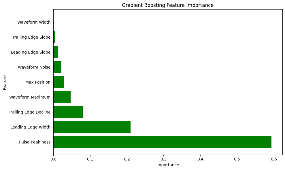
Gradient Boosting#
Implements a Gradient Boosting Classifier on waveform features, optimising misclassified samples.
Evaluates model performance using accuracy and classification metrics.
Ranks feature importance to identify the most influential waveform characteristics (e.g., Pulse Peakiness, Leading Edge Width).
XGBoost#
Trains an XGBoost Classifier using engineered waveform features, leveraging regularised gradient boosting.
Evaluates model performance using accuracy and classification metrics.
Ranks feature importance to identify the most influential waveform characteristics (e.g., Pulse Peakiness, Leading Edge Width).
import numpy as np
import pandas as pd
import matplotlib.pyplot as plt
from sklearn.model_selection import train_test_split
from sklearn.preprocessing import StandardScaler
from sklearn.metrics import accuracy_score, classification_report, confusion_matrix, roc_curve, auc
import seaborn as sns

# Function to plot feature importance overlaid on average waveforms
def plot_importance_on_waveform(feature_importance, model_name, X_clean, y_clean):
    plt.figure(figsize=(15, 6))

    # Plot average waveforms
    waveforms_class0 = X_clean[y_clean == 0]
    waveforms_class1 = X_clean[y_clean == 1]

    if len(waveforms_class0) > 0:
        plt.plot(np.mean(waveforms_class0, axis=0), 'b-', label='Lead (Class 0)', alpha=0.5)
    if len(waveforms_class1) > 0:
        plt.plot(np.mean(waveforms_class1, axis=0), 'r-', label='Sea Ice (Class 1)', alpha=0.5)

    # Scale importance for visualization
    max_wave_amp = max(
        np.max(np.mean(waveforms_class0, axis=0)) if len(waveforms_class0) > 0 else 0,
        np.max(np.mean(waveforms_class1, axis=0)) if len(waveforms_class1) > 0 else 0
    )

    if max(feature_importance) > 0:  # Avoid division by zero
        importance_scaling = max_wave_amp / max(feature_importance) * 2
        plt.bar(range(len(feature_importance)),
                feature_importance * importance_scaling,
                alpha=0.3,
                color='g',
                label='Feature Importance')

    plt.title(f'{model_name}: Feature Importance vs. Waveform Patterns')
    plt.xlabel('Sample Index')
    plt.ylabel('Amplitude / Importance')
    plt.legend()
    plt.grid(True, alpha=0.3)
    plt.show()
from sklearn.ensemble import RandomForestClassifier

print("=== Training Random Forest Classifier with Waveform Features ===")
rf_model = RandomForestClassifier(
    n_estimators=100,
    max_depth=20,
    min_samples_split=5,
    min_samples_leaf=2,
    random_state=42,
    class_weight='balanced'
)

# Train the model on extracted features
rf_model.fit(X_train_scaled, y_train)

# Make predictions
y_pred_rf = rf_model.predict(X_test_scaled)
y_pred_prob_rf = rf_model.predict_proba(X_test_scaled)[:, 1]

# Evaluate
accuracy_rf = accuracy_score(y_test, y_pred_rf)
print(f"Random Forest Accuracy: {accuracy_rf:.4f}")
print("\nClassification Report:")
print(classification_report(y_test, y_pred_rf))

# Get feature importance
feature_importance_rf = rf_model.feature_importances_

# Create feature importance visualization
plt.figure(figsize=(10, 6))
importance_df = pd.DataFrame({
    'Feature': feature_names,
    'Importance': feature_importance_rf
}).sort_values('Importance', ascending=False)

plt.barh(importance_df['Feature'], importance_df['Importance'], color='skyblue')
plt.xlabel('Importance')
plt.ylabel('Feature')
plt.title('Random Forest Feature Importance')
plt.tight_layout()
plt.show()
=== Training Random Forest Classifier with Waveform Features ===
Random Forest Accuracy: 0.9749

Classification Report:
              precision    recall  f1-score   support

           0       0.80      0.63      0.70       121
           1       0.98      0.99      0.99      2432

    accuracy                           0.97      2553
   macro avg       0.89      0.81      0.85      2553
weighted avg       0.97      0.97      0.97      2553
from sklearn.ensemble import GradientBoostingClassifier

print("=== Training Gradient Boosting Classifier with Waveform Features ===")
gb_model = GradientBoostingClassifier(
    n_estimators=100,
    learning_rate=0.1,
    max_depth=5,
    min_samples_split=10,
    random_state=42
)

# Train the model on extracted features
gb_model.fit(X_train_scaled, y_train)

# Make predictions
y_pred_gb = gb_model.predict(X_test_scaled)
y_pred_prob_gb = gb_model.predict_proba(X_test_scaled)[:, 1]

# Evaluate
accuracy_gb = accuracy_score(y_test, y_pred_gb)
print(f"Gradient Boosting Accuracy: {accuracy_gb:.4f}")
print("\nClassification Report:")
print(classification_report(y_test, y_pred_gb))

# Get feature importance
feature_importance_gb = gb_model.feature_importances_

# Create feature importance visualization
plt.figure(figsize=(10, 6))
importance_df = pd.DataFrame({
    'Feature': feature_names,
    'Importance': feature_importance_gb
}).sort_values('Importance', ascending=False)

plt.barh(importance_df['Feature'], importance_df['Importance'], color='green')
plt.xlabel('Importance')
plt.ylabel('Feature')
plt.title('Gradient Boosting Feature Importance')
plt.tight_layout()
plt.show()
=== Training Gradient Boosting Classifier with Waveform Features ===
Gradient Boosting Accuracy: 0.9738

Classification Report:
              precision    recall  f1-score   support

           0       0.80      0.60      0.68       121
           1       0.98      0.99      0.99      2432

    accuracy                           0.97      2553
   macro avg       0.89      0.79      0.83      2553
weighted avg       0.97      0.97      0.97      2553
import xgboost as xgb

print("=== Training XGBoost Classifier with Waveform Features ===")
xgb_model = xgb.XGBClassifier(
    n_estimators=100,
    max_depth=5,
    learning_rate=0.1,
    use_label_encoder=False,
    eval_metric='logloss',
    random_state=42
)

# Train the model on extracted features
xgb_model.fit(X_train_scaled, y_train)

# Make predictions
y_pred_xgb = xgb_model.predict(X_test_scaled)
y_pred_prob_xgb = xgb_model.predict_proba(X_test_scaled)[:, 1]

# Evaluate
accuracy_xgb = accuracy_score(y_test, y_pred_xgb)
print(f"XGBoost Accuracy: {accuracy_xgb:.4f}")
print("\nClassification Report:")
print(classification_report(y_test, y_pred_xgb))

# Get feature importance
feature_importance_xgb = xgb_model.feature_importances_

# Create feature importance visualization
plt.figure(figsize=(10, 6))
importance_df = pd.DataFrame({
    'Feature': feature_names,
    'Importance': feature_importance_xgb
}).sort_values('Importance', ascending=False)

plt.barh(importance_df['Feature'], importance_df['Importance'], color='red')
plt.xlabel('Importance')
plt.ylabel('Feature')
plt.title('XGBoost Feature Importance')
plt.tight_layout()
plt.show()
=== Training XGBoost Classifier with Waveform Features ===
/usr/local/lib/python3.11/dist-packages/xgboost/core.py:158: UserWarning: [16:53:31] WARNING: /workspace/src/learner.cc:740:
Parameters: { "use_label_encoder" } are not used.

  warnings.warn(smsg, UserWarning)
XGBoost Accuracy: 0.9745

Classification Report:
              precision    recall  f1-score   support

           0       0.84      0.57      0.68       121
           1       0.98      0.99      0.99      2432

    accuracy                           0.97      2553
   macro avg       0.91      0.78      0.83      2553
weighted avg       0.97      0.97      0.97      2553